THE GOAL
For this post, we will be looking at our visualizations and seeing what kind of stories and information we can glean from them. I have included the source code for these visualizations on this page, but as the big chunks of code ruined the flow of visualizations and analysis most of it is folded. If you so desire to see it, then merely click the “fold-outs” labelled Code and you can analyze away. :)
The Question
As I was perusing our data frame, the overall statistic began to seem more and more arbitrary. Some players with a wide, even spread of stats had a far lower overall than another player with high values in a few stats and lower values everywhere else. This got me wondering about how a player’s overall is really calculated as it is certainly not just the average of their stats. Let’s try to reverse engineer how the overall stat is really calculated
Visualizations
We’ll start by taking a look at the correlation coefficients each stat has in relation to a player’s overall rating. This will give us an idea of which stats most heavily influence all players’ overall ratings.
Code
```{python}
#Convert overall to int, add to player stats df, create correlation heatmap
combined_df = fifa_stats_df.join(players_dataframe["overall"])
corrmat = combined_df.corr()
f, ax = plt.subplots(figsize=(9, 9))
sns.heatmap(corrmat, square=True)

```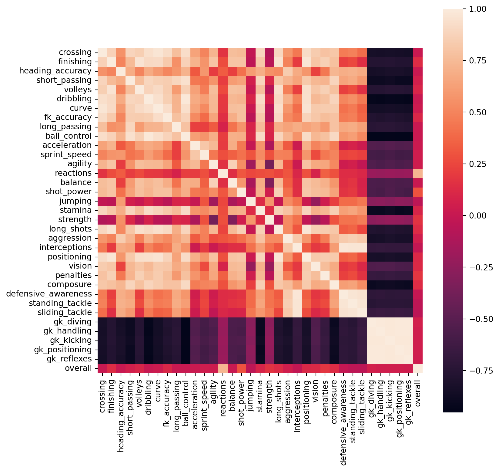
This chart is a bit overwhelming and doesn’t tell us much. Since we are really just interested in the stats that MOST influence the overall stat, let’s look at what 10 variables have the highest correlation coefficients with the “Overall” stat.
Code
```{python}
#Find the 10 highest correlations to overall, plot them on radar chart
cols = corrmat.nlargest(10, "overall")["overall"].index
ccm = np.corrcoef(combined_df[cols].values.T)
hm = sns.heatmap(ccm, cbar=True, annot=True, square=True, fmt=".2f", annot_kws={"size":10}, yticklabels=cols.values, xticklabels=cols.values)
plt.show()
```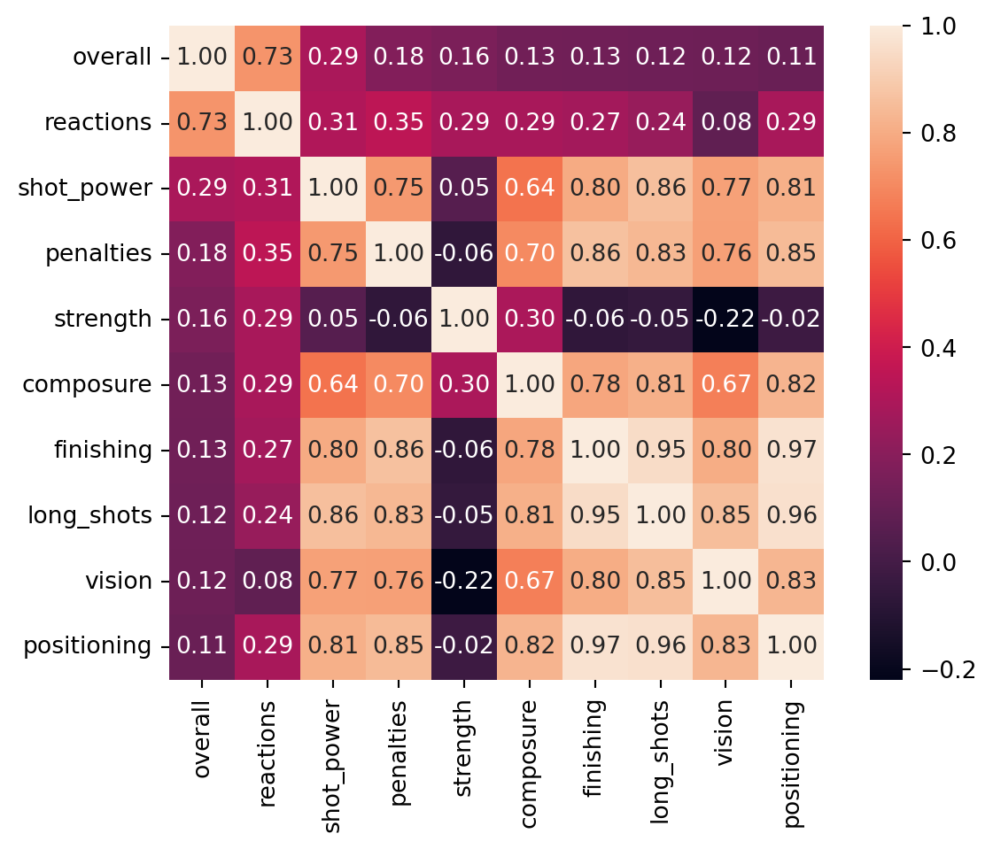 Looking at this chart we can see that interestingly enough, Reactions is by far and wide the most correlated to a player’s overall. My guess is that this is simply because reactions is a stat that can be equally useful and utilized by players in all positions. This leads me to the hypothesis that a player’s overall is determined not only by their stats, but also by their stats in relation to their position.
This would mean that if two players had the same exact stats, both of which are very talented at defense, the player that plays in a more defensive position would have a higher overall. This hypothesis is lent strong supported by the overall stat of goalkeepers, as their overall ratings would be extremely low if all stats impacted overall the same. However of the 60 players I grabbed, there are a number of keepers present on the list with rather high overalls. My curiosity lies in how much position affects what stats most strongly correlate to a player’s overall. Let’s do some exploration and see what we can find out.
First we will want to separate our players into offensive and defensive players. We can do this by sorting them by position. I elected to only use a select few positions as many midfield or outside players play all over the pitch and act as both defense and offense. In order to get the clearest picture of the correlations for offense vs defense, I chose positions that deal almost exclusively with either attacking or defending. Namely the attacking positions selected are striker, left and right wing, and the defense positions are center, left and right back.
Code
```{python}
#First we must narrow down our selections to offensive (Position is ST,RW,LW) and defensive players (Position is CB,RB,LB).
offensive_players = player_stats_df[
(player_stats_df["position_1"] == "ST") |
(player_stats_df["position_1"] == "RW") |
(player_stats_df["position_1"] == "LW")]
defensive_players = player_stats_df[
(player_stats_df["position_1"] == "CB") |
(player_stats_df["position_1"] == "RB") |
(player_stats_df["position_1"] == "LB")]

#Remove non int values for correlation coefficient calculation
offensive_players.drop(["last_name", "age", "potential", "team", "wage", "value", "stats", "id", "position_1", "position_2", "position_3", "contract_start", "contract_end"], axis=1, inplace=True)
defensive_players.drop(["last_name", "age", "potential", "team", "wage", "value", "stats", "id", "position_1", "position_2", "position_3", "contract_start", "contract_end"], axis=1, inplace=True)

off_corrmat = offensive_players.corr()
def_corrmat = defensive_players.corr()

#Create Offensive heatmap
cols = off_corrmat.nlargest(10, "overall")["overall"].index
ccm = np.corrcoef(offensive_players[cols].values.T)
hm = sns.heatmap(ccm, cbar=True, annot=True, square=True, fmt=".2f", annot_kws={"size":10}, yticklabels=cols.values, xticklabels=cols.values)
plt.show()

#Create defensive heatmap
cols = def_corrmat.nlargest(10, "overall")["overall"].index
ccm = np.corrcoef(defensive_players[cols].values.T)
hm = sns.heatmap(ccm, cbar=True, annot=True, square=True, fmt=".2f", annot_kws={"size":10}, yticklabels=cols.values, xticklabels=cols.values)
plt.show()
```
10 highest correlation coefficients for offensive players 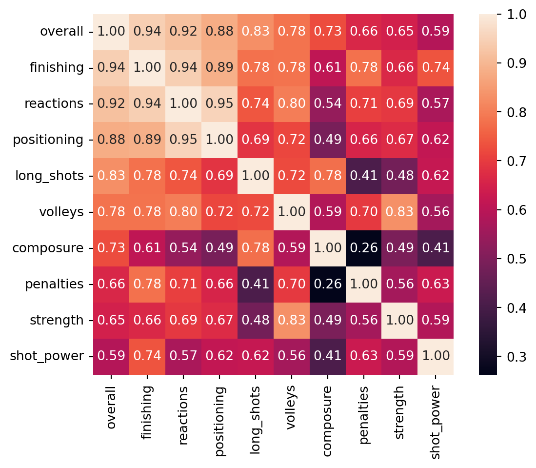 10 highest correlation coefficients for defensive players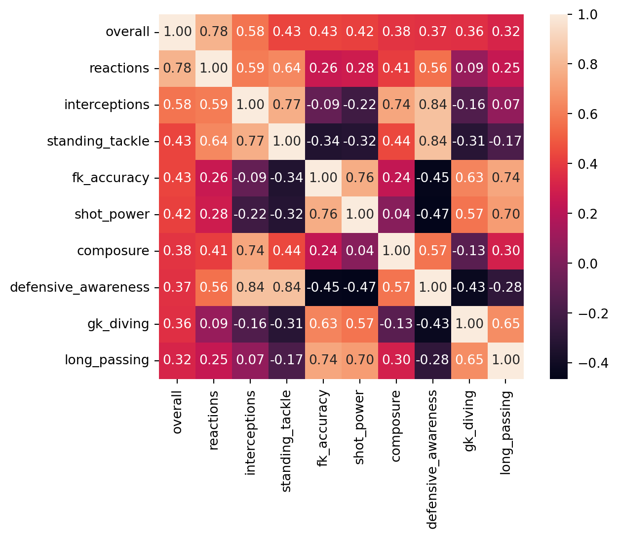
From this, it is easy to see that position severely influences the stats that have the most impact on a player’s overall. Many of the valued offensive stats are rather unsurprising, however I did not expect shot_power to have as little impact as it does. The real surprises lie in the Defensive players’ heatmaps. Defensive awareness has surprisingly little impact, lying under both shot power and free kick accuracy. One would think this skill invaluable for a player who’s primary task is to defend, so its low correlation coefficient is surprising to say the least. Not to mention that both shot power and free kick accuracy hold an unexpected amount of influence on a defensive player’s overall.
One can also observe that in general, the correlation coefficients of a defensive player are much lower than the correlation coefficients of an offensive player. Shot power for an offensive player, while having the lowest correlation of observed stats, still has a stronger correlation than interceptions for a defensive player, which has the second strongest correlation of all observed stats for defensive players and is a vital skill for anyone on defense. This suggests that offensive player overalls are inflated by a select few stats due to their high correlation coefficients, while a defensive player must be much more evenly spread across all stats in order to achieve a similar overall.
In order to test, this I would like to use spider plots. We can group statistics into various categories of offensive, defensive, passing, etc. This will give us an idea of a player’s capabilities in that category. From here, we will be able to compare spider plots and see if a defensive player’s stats are much more evenly spread than that of an offensive player.
For our categories, I decided on the following:
attacking
passing
physicality
pace
dribbling
mentality
defending
goalkeeping
You can see the breakdown of what stats go into each category in the block below.
Code
```{python}
#for usage later in dataframe
names = ["attacking", "passing", "physicality", "pace", "dribbling", "mentality", "defending", "goalkeeping"]


#Create function to make categories for player, return categories as list
def radar_plot_cats(dataframe):

  average = [0, 0, 0, 0, 0, 0, 0, 0]
  #First assign values to a list, then map them as INT, then get mean. Repeat for every point of radar plot
  attacking_col = [dataframe["finishing"], dataframe["heading_accuracy"], dataframe["volleys"], dataframe["shot_power"], dataframe["long_shots"]]
  attacking_col = list(map(int, attacking_col))
  average[0] = np.mean(attacking_col)

  passing_col = [dataframe["short_passing"], dataframe["long_passing"], dataframe["crossing"], dataframe["fk_accuracy"]]
  passing_col = list(map(int, passing_col))
  average[1] = np.mean(passing_col)

  physicality_col = [dataframe["reactions"], dataframe["balance"], dataframe["strength"], dataframe["jumping"]]
  physicality_col = list(map(int, physicality_col))
  average[2] = np.mean(physicality_col)

  pace_col = [dataframe["acceleration"], dataframe["sprint_speed"], dataframe["agility"]]
  pace_col = list(map(int, pace_col))
  average[3] = np.mean(pace_col)

  dribbling_col = [dataframe["dribbling"], dataframe["ball_control"]]
  dribbling_col = list(map(int, dribbling_col))
  average[4] = np.mean(dribbling_col)

  mentality_col = [dataframe["aggression"], dataframe["positioning"], dataframe["vision"], dataframe["composure"]]
  mentality_col = list(map(int, mentality_col))
  average[5] = np.mean(mentality_col)

  defending_col = [dataframe["interceptions"], dataframe["defensive_awareness"], dataframe["standing_tackle"], dataframe["sliding_tackle"]]
  defending_col = list(map(int, defending_col))
  average[6] = np.mean(defending_col)

  goalkeeping_col = [dataframe["gk_diving"], dataframe["gk_handling"], dataframe["gk_kicking"], dataframe["gk_positioning"], dataframe["gk_reflexes"]]
  goalkeeping_col = list(map(int, goalkeeping_col))
  average[7] = np.mean(goalkeeping_col)

  return average
```
```{python}
selected_player = player_stats_df.loc[0]
player_cat = radar_plot_cats(selected_player)
#Create dataframe for plot
data_dict = {"names": names, "average": average}
df = pd.DataFrame(data_dict)
#Create and show graphs for selected player
fig = px.line_polar(df, r="average", theta ="names", line_close=True)
fig.update_traces(fill="toself")
print("Player:", selected_player["last_name"],",", "Overall:", selected_player["overall"],",", "Position:", selected_player["position_1"])
fig.show()
```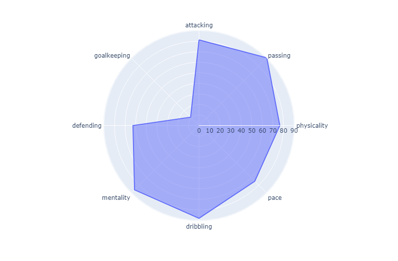 Here is the spider plot for Kevin Debruyne. He is a midfielder who is known for his prolific assisting and an incredible passing game. I wanted to show this plot as a benchmark for ones that follow. Once again, keep in mind that this is one of the current best players in the world who is known for his attacking prowess through setting up attacking opportunities.
Below are two radar plots overlaid on top of one another. I have chosen Erling Haaland, the most prolific scorer from last season and Virgil Van Dijk, who is believed to be the best defender in the premier league for these plots.
Code
```{python}
#For Van Dijk (defensive)
def_cat = radar_plot_cats(player_stats_df.loc[6])
#For Haaland (offensive)
off_cat = radar_plot_cats(player_stats_df.loc[1])
#Create new lists for usage in dataframe to create two radar plots on top of each other
cat_value = off_cat + def_cat
names = names + names[:]
group = ["Haaland (Offense)", "Haaland (Offense)", "Haaland (Offense)", "Haaland (Offense)", "Haaland (Offense)", "Haaland (Offense)", "Haaland (Offense)", "Haaland (Offense)",
"Van Dijk (Defense)", "Van Dijk (Defense)", "Van Dijk (Defense)", "Van Dijk (Defense)", "Van Dijk (Defense)", "Van Dijk (Defense)", "Van Dijk (Defense)", "Van Dijk (Defense)"]
#Create dataframe for plot
data_dict = {"names": names, "average": cat_value, "group": group}
df = pd.DataFrame(data_dict)
#Create and show graphs for selected player
fig = px.line_polar(df, r="average", theta="names", line_close=True, color="group")
fig.update_traces(fill="toself")
fig.show()
```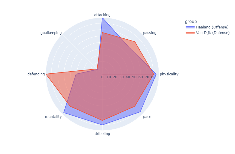 Here we can actually see the opposite of what I expected to observe. It looks like Haaland has a better spread of stats, even though he is an offensive player. It should also be noted that Haaland has an overall of 90, while Van Dijk has an overall of 88. Perhaps a better measurement would be to compare an offensive and defensive player who have the same overall, so we shall see what happens when we try that. It uses the same code as above, with the only difference being the reference indices used in the function.
For this next comparison, I will use Son Heung-Min, an 88 rated Left Winger and Ruben Dias, an 88 rated Center back.
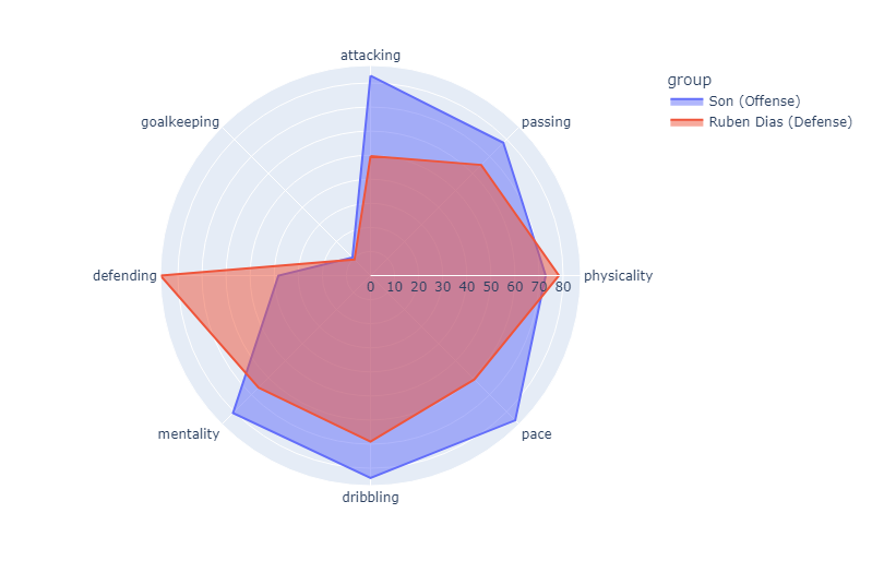 Interesting enough, this plot looks almost the exact same as the last. We can see that unsurprisingly, our defensive player has much higher defensive stats than our offensive player and our offensive player has higher attacking stats than our defensive player. Our offensive player also beats out our defensive player in every category other than physicality and defending. Perhaps the issue lies with my categories for the plots for example, they may favor an offensive player’s play style rather than that of defense. One way we can get around this is by simply observing the mean of their stats, as this will give us an idea of their average numbers.
Code
```{python}
# filter out outliers (such as low goalkeeping stats)
lower_limit = 40
upper_limit = 99

# Filter values within the specified range for Ruben Dias (defensive)
filtered_values = fifa_stats_df.iloc[9].loc[(fifa_stats_df.iloc[9] >= lower_limit) & (fifa_stats_df.iloc[9] <= upper_limit)]
mean_value = filtered_values.mean()

print(mean_value)

# Filter values within the specified range for Son (offensive)
filtered_values = fifa_stats_df.iloc[10].loc[(fifa_stats_df.iloc[10] >= lower_limit) & (fifa_stats_df.iloc[10] <= upper_limit)]
mean_value = filtered_values.mean()

print(mean_value)
```
Running this code means we can see the following:
| player | average | overall | position |
|---|---|---|---|
| Haaand | 76.79 | 90 | ST |
| Son | 79.19 | 88 | LW |
| Van Dijk | 73.57 | 88 | CB |
| Ruben Dias | 71.84 | 88 | CB |
| DeBruyne | 80.40 | 91 | CM |
This is rather interesting. Not only do our offensive players have higher average stats, but our 90 rated offensive player has a whopping 2.5 lower average stat, even though his overall is 2 points higher than our our other offensive player. Let’s take a closer look at this difference. 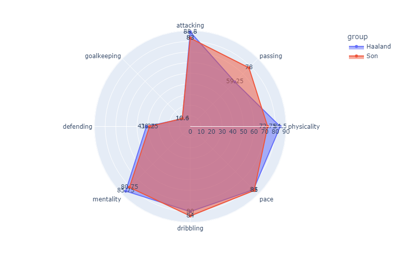 It seems that most of this difference comes down to the attacking category, as our correlation matrix shows how large of an influence these stats in that category have on an attacking player’s overall. Son’s passing stats average is almost 20 points higher than those of Haaland’s, with most of the other categories being neck and neck save for the physical stats. This stark difference simply shows how much influence a player’s position has for the determining their overall.
This leaves our defensive players. Their stats are on average lower than those of their offensive player counterparts. There are likely a number of explanations for this effect, however I believe it to be due mostly to the measured stats that Fifa collects.
While offensive players have 6 different stats just for different types of shots (finishing, volleys, long shots, shot power, penalties and free kick accuracy), there are only 3 stats in total that are defensive in nature, two of which are simply different types of tackles. This gives offensive players many more ways to bring up their average stats by working only on attacking stats, whereas defensive players are constricted largely to their three defense stats. This is not to mention that many of the other stat categories such as dribbling or pace have seemingly little use to defenders, as their job is mostly to simply clear threats by clearing the ball up the field or out of play.
This gives defensive players a rather linear and 1-dimensional way of play, at least in the frame of fifa stats. In reality, there are a number of players that break out of this frame, such as Trent Alexander Arnold or Virgil Van Dijk, both of which are renowned as excellent crossers/passers and frequently finish games with an assist or a key pass that leads to an attacking opportunity. However due to their low correlation coefficients, these stats do little to impact their overall. This leaves their overall stagnant, even though they are a significant boon to their team’s play. This is a fault of Fifa’s data collection. By giving these stats a low correlation coefficient, this undermines the player’s overall and value to a team.
Conclusion
So what does this mean for our original hypothesis, that offensive player overalls are inflated by a select few stats due to their high correlation coefficients, while a defensive player must be much more evenly spread across all stats in order to achieve a similar overall. Seeing that offensive players often had higher overall stats and more even spreads than their defensive counterparts, our original hypothesis was disproved.
This implies an overall bias towards offensively-oriented players. It is much easier for an offensive player to improve their overall as long as they improve in their attacking stats, than it would be for a defensive player to improve their overall by working solely on their defensive stats. A player who is a perfect attacker, with a 99 in all stats in the attacking category and 0’s everywhere else, would have a SIGNFICIANTLY higher overall than a player who is a perfect defender with a 99 in defending stats and a 0 for everything else.
This data shows a rather disappointing lack of appreciation for the art of defense. This is a rather common precedent in the world of professional soccer, with there being 66 Ballon’D’Or awards since its inception in 1956, only 4 of which have ever gone to a defensive player. The world of soccer has created a very superficial idea of what it means to be a defensive player, deeming that their role is simply to defend. In reality, there is so much more depth in how they can contribute and create opportunities for their team. Fifa, as well as the soccer world in general, should recognize how much more defensive players have to offer than merely “defense”. Players like Marcelo, Trent Alexander Arnold and Virgil Van Dijk continue to push the envelope and show the world how much more a defender can contribute to a team than just keeping the ball away from the net. Overall ratings should reflect how much one can contribute to their team’s success, rather than simply fill a role/position. Dynamic players who fill multiple roles should be rewarded with a higher overall, not penalized for their inadequacies in one singular statistic.